

This post is a collection of learnings around contextual bandits. At Ravelin, we use these techniques to optimise transaction conversion rates.
I’ll highlight some methods for evaluating bandit policies both offline & online along with the unique challenges they present—challenges that don’t typically arise in fully supervised learning, which is what makes it interesting!
Many applications require you to optimise decisions where there are multiple options — like choosing web designs, email templates, or product recommendations. You want to learn what works best and continue to improve, while still delivering good results along the way. That’s where contextual bandit policies shine!
What is a contextual bandit model?
Multi-armed bandits (MAB) are a type of reinforcement learning framework – a field of machine learning where agents learn optimal behaviours by taking actions and receiving feedback from their environment. MAB describes a subset of problems where the agent earns a reward immediately after taking an action and there are no states or state transitions.
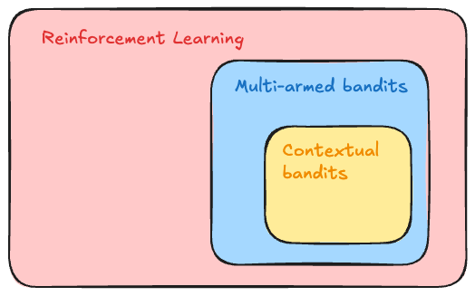
The contextual bandit problem extends the multi-armed bandit framework by incorporating contextual information (features) to make decisions. That means trials with different feature sets can lead to different reward estimates; an action that is optimal for one trial may not be optimal for another.
This kind of problem appears way more often in the real world than you might expect!
- optimising treatment allocation in clinical trials
- website click-through-rate optimisation
- artwork personalisation at Netflix
At Ravelin, we use the contextual bandits framework to optimise transaction conversion rates, by routing transactions to maximise the likelihood of authorisation by the issuing bank.
For our use case, the theory can be mapped onto practice as follows:
- The “arm” (also called the “treatment” or the “action”), is one of K different transaction routing options (for example what authentication exemptions or challenge preferences to apply)
- The “reward” is whether or not the transaction was successfully authorised — a binary 0/1 signal (this can be extended to more complex rewards)
- The “context” is all of the machine learning features we have at our disposal
Ultimately, in contextual bandits you want to use the context and labels to predict the reward for each of the K arms. This is a bit like a multi-label classification where there are multiple output predictions, as in the image below.
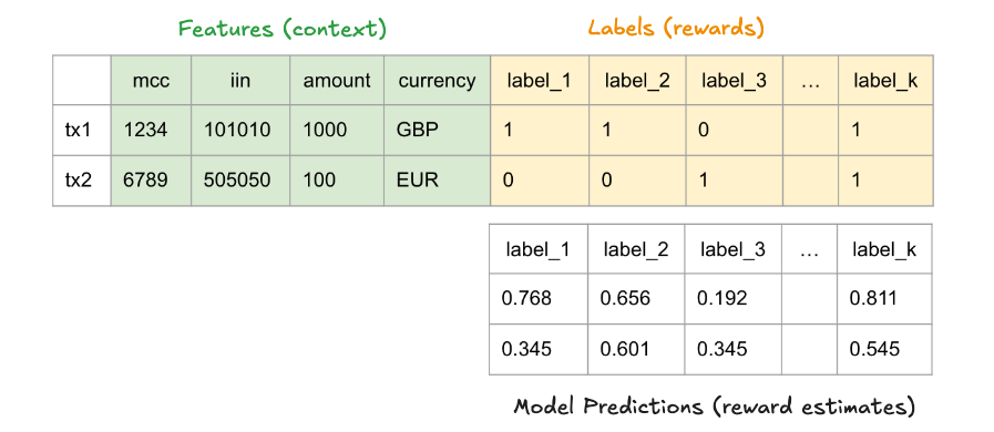
OK, so what makes this problem different from supervised learning?
Labels are only partially known!
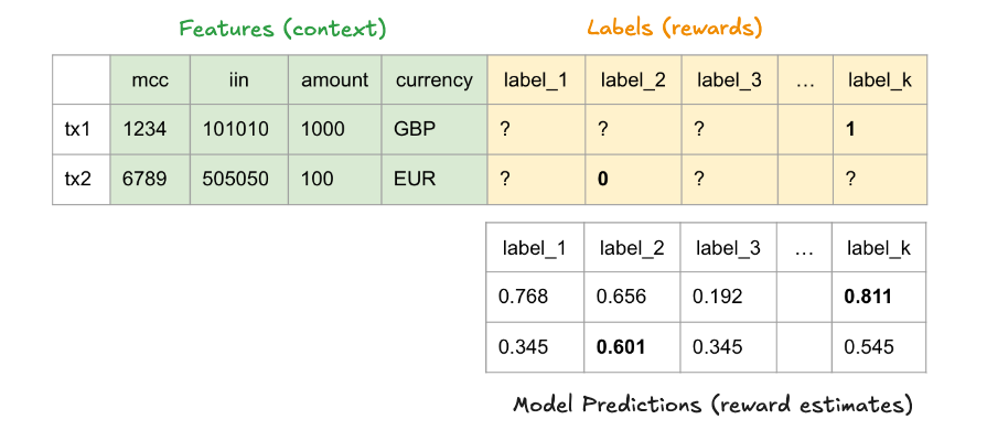
Once you’ve decided that you want to pull a particular arm, you take action and your environment returns a reward. Very rarely in the real world can you go back and “try again”. Once an action has been performed, you cannot know what would have happened down had you chosen a different action.
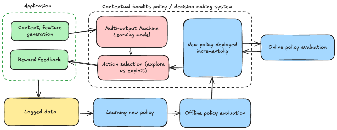
For the rest of the bandits recommendation system, you also need to decide on the following two things:
- whether you want to train the model online (on-policy learning) or offline (off-policy learning) [1]
- how you want to explore (this is the exploration vs exploitation tradeoff fundamental to any reinforcement learning problem). This can be a function of the model outputs.
With all of these things decided, you can define your reinforcement learning policy.
What’s a policy?
A policy is the strategy or decision-making rule used to determine the actions we’ll choose at each step. It’s almost always a stochastic policy, meaning a probability distribution over the available actions.
Let’s assume you’ve got a model which outputs K probabilities, one for each arm. After applying the exploration policy, you are left with a distribution of selection probabilities over your K arms which always add up to 1. You pull one of the arms probabilistically from this final distribution at each step.
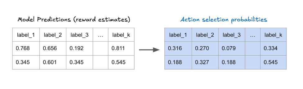
For example, imagine you’re using an epsilon-greedy policy with epsilon = 0.1. Then the model outputs and action selection probabilities might look something like this:
- Model outputs (number of actions k=5):
![[0.768, 0.656, 0.192, 0.811, 0.122]](https://olliesmith.blog/wp-content/ql-cache/quicklatex.com-e7cfe3ed59e20f0a3f333a75cb630ade_l3.png "Rendered by QuickLaTeX.com")
- Action Selection Probabilities:
![[0.025, 0.025, 0.025, 0.9, 0.025]](https://olliesmith.blog/wp-content/ql-cache/quicklatex.com-bd26cd4d2bc3e8739b56e9266062f918_l3.png "Rendered by QuickLaTeX.com")
This is because a 90% chance is assigned to the “best” action (the highest output: 0.811), and the remaining 10% is equally distributed among the other actions.
For the rest of this article I’ll assume we’ve trained a model using off-policy learning, and have chosen a reasonable exploration strategy. For on-policy learning I’d check out this paper which has a few potential options.
Now that we understand what a policy is and how it makes decisions, the crucial question becomes: how do we know if our new policy is actually better than the current one? Unlike traditional machine learning models where we can directly measure performance on a test set, evaluating bandit policies presents unique challenges that require special techniques.
Evaluating contextual bandit policies
Normally when we train a supervised model, we are able to split the dataset into train and test sets and assuming all is well, the performance metrics on the test set will a good idea of how the model will perform on unseen data in the future. But when there’s partial feedback involved, this is more difficult.
A natural metric is the “average reward” under the new policy. The problem is that the process which collected the data is different to the process that will select actions in the future, once you’ve deployed the model to production.
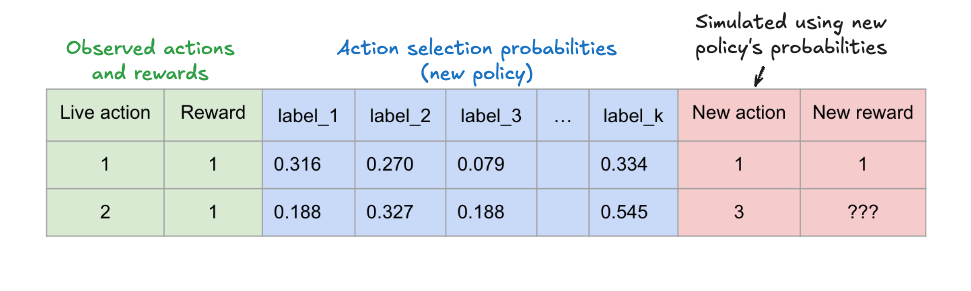
We only know whether the new policy’s action would’ve been a good one if it matches the action chosen by the live policy. And only evaluating the average expected reward on those rows where the two policies match (dropping all rows where they don’t match) introduces bias. This means that we cannot trust such metrics to generalise to unseen data in the future, when the new policy will be making the decisions.
Off-policy evaluation techniques
Even though we’ll never know what rewards the new policy’s actions would have revealed on our partially-labelled dataset, we can still use the old data to come up with unbiased estimates of our new policy’s performance. These are well-known causal inference techniques, which are relevant here as we are estimating the counterfactual of what would have happened under a different policy.
This Medium article talks in more detail about the methods outlined below and also talks about the ways Facebook have used offline policy evaluation as part of their A/B testing platform. I also found this paper a very useful reference point for checking that these estimators are indeed unbiased.
Note: For off-policy evaluation techniques, you need to know what the action selection probabilities were under the live policy too!
Inverse Propensity Scoring (IPS)
Firstly some notation, let  be the new policy’s action selection probabilities and let
  be the old (live) policy.
  is the reward observed by the live policy,
  is the action taken by the live policy, and
  is the context (features) at each step
  .
.
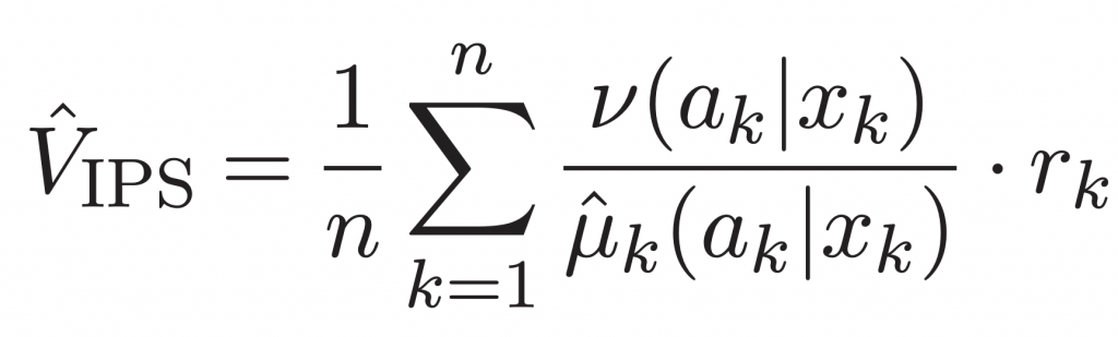
Here’s an intuition behind the IPS estimate:
- we are taking a weighted average of the rewards seen at each step. The weights are given by

- the
 term acts as a debiasing factor, to account for the fact that the way the data was gathered is biased towards the live policy’s preferences
 - the
 term is in the numerator because, what we ultimately want is an expected value
  under the new policy’s probabilities
This paper [3] demonstrates that IPS is an unbiased estimate for the true expected reward under the new policy.
Doubly Robust (DR)
This method does the following:
- First build a predictive model for the new policy’s reward, given context and action, using historical data. This is called the reward model. Training a separate reward model for offline policy evaluation might seem circular at first glance, but it serves a specific purpose. Reward models are an important component in RLHF used to make LLMs perform better at their tasks.
- Once you’ve fitted a reward model, you then take the average across your logged policy’s rows of this reward estimate.
- Take the reward estimates and combine them in a clever way with the IPS estimates — see the paper for DR for the juicy details, I won’t go into it here.
It can be shown that the DR method is a strict improvement upon the IPS method! This is likely worth it for reliable inference, if you’re happy with the extra complexity of training a reward model for the new policy!
There are implementations of both IPS and DR offline policy estimation in this repo.
Online evaluation and A/B testing
Given enough data, the offline techniques above should give you enough confidence that the policy you’re about to deploy will perform better than whatever live policy is currently in place.
But we should be wary of the practical limitations of these offline evaluation estimates:
- sample size issues — lesser explored actions have much lower probabilities of being chosen, and if your new policy is frequently picking those then this will add more variability to the weighted reward estimates
- drift — the live policy could have logged the data over a long time period over which changes in the underlying environment may have occurred
For this reason I would also advocate for also evaluating online. And by that, I mean putting the model live and seeing what happens, gathering the new policy’s feedback as you go. This sounds scary, but the risks can be minimised by rolling out the new model recommendations on a small portion of traffic initially (say, 1%, 5% or 10%) and scale up after gathering rewards from the new policy’s actions. This is, essentially, an A/B test between your old policy and your new policy.
If you have good monitoring in place, you should be able to see quickly whether the new model’s recommendations are providing as much uplift as you were expecting from your offline calculations.
The drawback, of course, of online evaluation is that testing online can be expensive. You’ve got to be pretty happy with your new policy before you start rolling it out on a small fraction of traffic, because if it’s worse than the current policy then you’ll have a detrimental effect on the real world. This is why offline evaluation should always be run first, before moving on to the online evaluation stage!
In addition to that, if you don’t have the right systems / technology / engineering infrastructure in place to be able to shift traffic between the old and new policies easily, it can also be a time consuming and painful experience.
Conclusion
There are perils when dealing with partial feedback. You are at the mercy of the data gathered from your current policy, and there are plenty of actions which are not taken for which we are blind.
By using some clever causal inference techniques, we can still come up with some pretty reliable estimates as to how much uplift your newly trained model will achieve.
However, there are drawbacks, and practically speaking you’ll want to roll out the model on live traffic gradually and regularly check that the uplift is as expected. You could automate all steps of this to make it a seamless model update using off-policy learning. This is the approach we have decided to take for transaction optimisation.
Resources
- [1] Chapter 2 of this book gives a nice formal introduction to multi-armed bandits: http://incompleteideas.net/book/RLbook2020.pdf
- [2] https://www.ericsson.com/en/blog/2023/12/online-and-offline-reinforcement-learning-what-are-they-and-how-do-they-compare
- [3] Offline Policy Evaluation in a Contextual Bandit Problem https://math.uchicago.edu/~may/REU2019/REUPapers/Kim,SangHoon.pdf
- [4] A very relevant article on Medium: E. Conti, Offline Policy Evaluation: Run fewer, better A/B tests
- [5] Doubly Robust Policy Evaluation and Optimization — https://arxiv.org/abs/1503.02834
- [6] Online contextual bandits modelling: https://arxiv.org/pdf/1811.04383